2 Pre-Processing and EDA
Once the raw data is acquired, it must be rigorously processed to ensure suitability for the machine learning pipeline. This phase includes cleaning data, handling missing values, encoding categorical variables, and analyzing feature distributions. Given the geospatial nature of our dataset, this step was crucial for ensuring that our grid-based predictions were accurate and not biased by noise.
2.1 Dataset Collection
Our dataset was constructed by aggregating multiple geospatial data sources to create a unified “grid” of the target urban area. The primary data sources included:
- OpenStreetMap (OSM): For road network data (primary, secondary, tertiary roads) and Points of Interest (POIs) such as commercial centers, residential complexes, and transport hubs.
- Demographic Data: Population density estimates mapped to grid cells.
- Traffic Data: Historical traffic volume estimates for major intersections.
The study area was divided into hexagonal/square grid cells, with each row in the dataset representing a specific geospatial location (identified by grid_id, latitude, longitude).
2.2 Data Pre-processing
Data pre-processing was an iterative process involving several key challenges and solutions.
2.2.1 1. Handling Missing Values
We encountered missing values primarily in peripheral grid cells where sensor data or POI density was sparse.
- Analysis: A pattern analysis showed that missing values were not random (MNAR); they clustered in low-density residential areas or open spaces.
- Solution: We employed Zero Imputation for POI counts (assuming null meant zero presence) and Median Imputation for continuous variables like
traffic_volumeto avoid skewing the distribution with outliers.
2.2.2 2. Encoding and Data Types (Key Challenge)
A significant challenge encountered during the pipeline development was the presence of non-numeric data types in the training set.
- Issue: The XGBoost algorithm threw specific
ValueErrorandAttributeErrorexceptions when encountering columns of typeobject(e.g.,grid_type,zone_name). - Solution: We implemented a strict filtering process to drop non-informative string columns. Categorical variables with predictive power were One-Hot Encoded, while purely descriptive text columns were removed from the input matrix
X_inferenceto resolveDataFrame.dtypesconflicts.
2.2.3 3. Scaling
While tree-based models like XGBoost are generally robust to unscaled data, we applied Min-Max Scaling to features like population_density and traffic_volume. This ensured that features with large raw values did not dominate the initial tree-building splits, although for the final XGBoost implementation, this step was less critical than for linear models.
2.2.4 4. Outliers
The dataset contained significant outliers, particularly in the poi_density_commercial feature (Central Business Districts).
- Decision: We chose not to remove these outliers. In the context of EV charging station placement, these “outliers” represent high-value targets (hotspots). Capping or removing them would have eliminated the very locations we aimed to identify.
2.3 Exploratory Data Analysis and Visualisations
We conducted EDA to understand the underlying structure of the urban environment and validate our feature engineering.
2.3.1 Data Visualization
We utilized histograms and box plots to analyze feature distributions.
- Observation: Most density features (e.g.,
poi_density_residential) followed a Power Law distribution (right-skewed), indicating that a small number of grid cells contain the majority of urban activity. - Action: This confirmed the need for a non-linear model like XGBoost, which handles skewed distributions better than standard regression.
2.3.2 Statistical Analysis
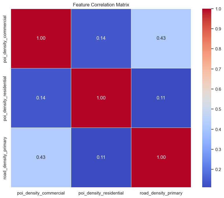
We computed a Correlation Matrix to identify relationships between variables.
- Findings: Strong multicollinearity was observed between
road_density_primaryandpoi_density_commercial. - Impact: While collinearity does not ruin prediction accuracy in boosted trees, it complicates feature importance interpretation. We noted this when analyzing the model’s “Feature Importance” output later.
2.3.3 Feature Selection and Dimensionality Reduction
We faced a “Feature Mismatch” issue where the inference dataset contained ~40 columns while the trained model expected only 6 specific features. This forced a rigorous feature selection process.
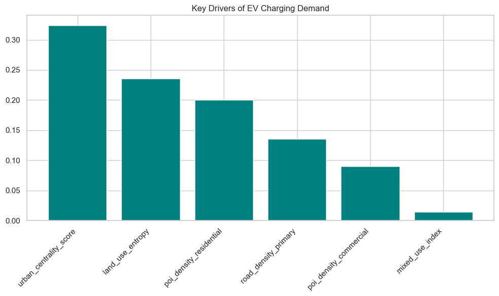
Using Recursive Feature Elimination (RFE) and domain knowledge, we narrowed our model down to the 6 most impactful predictors:
land_use_entropy(Measure of mixed-use development)poi_density_commercialpoi_density_residentialroad_density_primaryurban_centrality_scoremixed_use_index
This dimensionality reduction not only improved model training speed but also prevented the “Curse of Dimensionality,” ensuring the model focused on signal rather than noise.